Freefall Lab

Free Fall Lab: Determination of g 

Jin Im

with Juan Garcia

1 March, 2017

This lab was performed to determine the value of g by using the position of a falling object at precise time intervals.

Introduction: Using a "free fall" apparatus, we obtained the position of a falling spark generator at small, equal time intervals. Using the ∆x of each interval we can derived the velocity of the falling object with which we can make a mid-interval speed vs. mid interval time graph, the slope of which should lead us to the experimental value of the constant acceleration that the spark generator experiences while falling.

Procedure: The system is setup by feeding spark-sensitive tape along the height of the 1.86m apparatus (pictured below). The spark generator is rested at the top of the apparatus, held by an electromagnet and aligned with a wire "railing". When the magnet is switched off, the spark generator falls, making black marks on the spark-sensitive tape at set intervals.

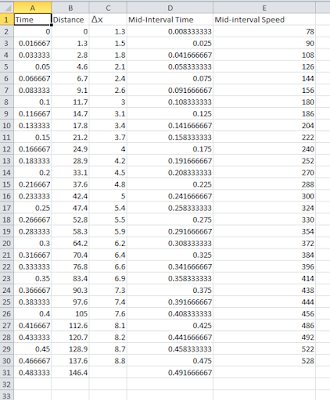
The spark tape is removed and the distance between each mark is measured. These values are our x. The values are input into an Excel sheet. On the same spreadsheet, we make cells for TIME (interval 1/60s), ∆x (difference between consecutive  values of x), mid-interval time (value of time + 1/120), and mid-interval speed (∆x/(1/60)). Then, we generated a mid-interval speed vs mid-interval time graph. The scatter point graph was linearly fit, and the slope should give us the experimental value of g.

Data:

Excel Data Table

Resulting Graph, Linear Fit

The Y-axis is the velocity of the falling spark generator in centimeters per second, while the X-axis is the time in seconds. The slope of this line represents the rate of change in V over time, or ∆v/t, which is the formula for acceleration. The line data shows us that the experimental value of acceleration is 969.69 cm/s^2 or 9.70 m/s^2.

Distance vs Time graph, Polynomial Fit

This graph is different from the first one in that the Y-axis is the value for distance in centimeters, so it becomes a distance vs time graph. The trendline is polynomial fit to the order of two: y=484.09x^2+68.843x-0.0103. This polynomial is in the form of the common kinematics equation 

y=v0t+0.5at^2. We can see that the value with the order of 2 represents 0.5 of a, and the experimental value 484.09 cm/s^2 is roughly half of the known value of g at 981 cm/s^2.

Class Data for g

The class data for this lab

The average class data for the experimental value of g was 961.5 cm/s^2 compared to our own 969.69 cm/s^2. Our standard deviation of the mean was 37.437, calculated by the formula below

Source: http://geographyfieldwork.com/StandardDeviation1.htm

Questions: 

1. Show that, for constant acceleration, the velocity in the middle of a time interval is the same as the average velocity for that time interval.

The velocities at the start of the time interval and the end of the time intervals are the velocities of interest, heretofore called Vi and Vf, respectively. Assuming constant acceleration, the change in velocities is linear and constant between Vi and Vf. That means the value of Vm at the middle of the time interval is equidistant from Vi and Vf  (Vm-Vi = Vf - Vm). Manipulating this equation yields 2Vm = Vf + Vi which yields Vm = (Vf-Vi)/2. Therefore, Vm = Vavg.

2. Describe how you can get the acceleration due to gravity from your velocity/time graph. Compare your result with the accepted value

Because acceleration is the rate of change in velocity over time, the slope of a velocity vs time graph is the value of g, in cm/s^2. Our experimental value of 969.69 cm/s^2 was slightly below the accepted value of 9.81m/s^2 or 981cm/s^2.

3. Describe how you can get the acceleration due to gravity from your position/time graph. Compare your result with the accepted value.

As mentioned above, position and acceleration are detached by an order of two. Using a polynomial trendline on our position vs time graph yielded us y = 484.09x^2+68.843x-0.0103. And because the kinematics formula with a relation between d, t, and a is x = v0t + 1/2(at^2), our value of g/2 is in the coefficient of the term in the second order. 484.09 * 2 = 968.18 cm/s^2, which is slightly lower than the accepted value of 9.81m/s^2.

Conclusion: 

Using the position data gathered from the "free fall" apparatus, we graphed both position vs time and velocity vs time in order to find our experimental value of g. We observed the relationship between position, time, velocity, and acceleration. Our experimental values of g, derived from both position and velocity graphs, were 969.69 cm/s^2 and 968.18 cm/s^2 respectively, slightly lower than the accepted value of 981 cm/s^2. This is most likely due to dissipative forces in the experiment: friction against the wire railing and a slight air resistance. These two forces counter act the force of the weight of the falling object, and the experiment is slightly flawed in that the object does not have an acceleration equal to the value of gravity. Our standard deviation of the mean from class data was 37.437.