06-March-2017 Propagated Uncertainty in Measurements

Density of Metal Cylinders and Propagated Uncertainty

Jin Im

with Victoria Bravo and Juan Garcia

6 March, 2017

In this lab, we observed the effects of uncertainty in everyday calculations and learned the significance of the range of values it provides.

Intro/Theory: We procured two cylinders of unknown composition. By taking their mass with a scale, and using calipers to find their volume, we calculated their densities. By comparing these values to a list of metals and their known densities, we found the identities of both cylinders.

Also, by using uncertainty values specific to the equipment used in the lab, we calculated the propagated uncertainty of each density calculation.

Procedure:  We retrieved 2 cylinders of unknown makeup and differing sizes. By weighing these cylinders on a scale, then measuring their dimensions with a caliper, we calculated their density in g/cm^3. We compared the resulting densities with the density values of known metal to find the identities of the metal cylinders.

Using the uncertainty from lack of precision in the equipment used today (d⌀, dh, and dm), we calculated the propagated uncertainty values of the densities of each cylinders and observed the range of the resulting values.

Data/Calculations: 

Cylinder 1: mass = 70.6g, height = 8.68 cm, diameter: 1.90 cm

Cylinder 2; mass = 28.9g, height = 3.25 cm, diameter: 1.28 cm

Because the scale measured mass to the tenths power, our uncertainty for mass was 70.6 ± 0.1g and 28.9 ± 0.1g, respectively.

Because the caliper measured to to to a hundredths of a centimeter, our uncertainty for each measurement was ± 0.01 cm. (8.68 ± 0.01 cm, 1.90 ± 0.01 cm / 3.25 ± 0.01 cm, 1.28 ± 0.01 cm).

The density formula is mass over volume, and the volume of a cylinder is 

V

=

π

r^2

h

replacing r for diameter/2, we get 

V

=1/4

πd^2

h.

Our density formula becomes 4m / 

πd^2

h.

Plugging in the values, Density of the large cylinder = 4(70.6) / [3.14(1.9/2)(8.68)] = 2.87 g/cm^3

Density of the smaller cylinder = 4(28.9) / [3.14(1.28/2)(3.25)] = 6.91 g/cm^3

The propagated uncertainty calculations are included below.

Conclusion: Our final densities of 2.87 ± 0.031g/cm^3 and 6.91 ± 0.0126 g/cm^3 where comparable to that of aluminum and zinc, respectively. Aluminum has a kg/m^3 density of 2712 and Zinc has 7135. Converting those quantities into g/cm^3, 2.712 and 7.135 are close enough to identify the two cylinders as aluminum and zinc. A possible source of discrepancy, however, would be the density of the hook at the top of each cylinder which we could not measure, and the impurity of the cylinders' makeups.

Lab 3: Non-constant acceleration problem/activity

Problem with a Non-constant Acceleration

Jin Im

6 March, 2017

In this lab, we explored how to solve, with Microsoft Excel, a kinematic equation in which the acceleration component was not constant -- normal kinematics equations do not apply. 

Introduction: A 5000 kg elephant on frictionless roller skates is going 15 m/s when it gets to the bottom of a hill and arrives on level ground. At that point a 1500 kg rocket mounted on the elephants back generates a constant 8000 N thrust opposite the elephant's direction of motion. The mass of the rocket changes with time (due to burning the fuel at a rate of 20 kg/s) so that the m(t) = 1500kg - 20kg/s*t. Find how far the elephant moves before coming to rest. 

We are given the analytical solution to this problem in the lab manual beforehand:

The answer to our problem is 248.7 meters. However, the process was very difficult and involved. The alternative way of solving this problem involves the use of Microsoft Excel, and is much faster.

Procedure: 

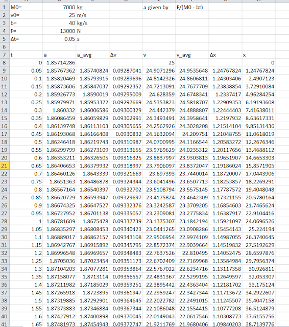
On our excel page, we attributed cells with static values including ∆t, initial mass, force, initial velocity, and fuel burn rate. We then created a row for dynamic values of elapsed time, acceleration, average(mid-point) acceleration, ∆v, velocity, average(mid-point) velocity, ∆x, and x. We set up these cells so they update with every row and time interval. 

Time was the previous value of time + ∆t.

Acceleration was the Force divided by the quantity for (Mass - burnrate*time).

Average acceleration was the mean of the accelerations at the beginning and the end of each time interval

∆v was average acceleration*∆t

Velocity was initially 25 m/s and reduced by ∆v for every time interval

Average velocity is the mean of the velocities in the beginning and end of each time interval

∆x is average velocity*∆t

x is the sum of all ∆x's.

The result is a spreadsheet like such:

Because we are interested in how far the elephant travels before coming to a stop, we can look at the t in which the velocity hits zero. From this, we can conclude from this data that the elephant stops moving by virtue of its initial motion between 19 and 20 seconds, and starts to move backwards due to the rocket, shown by the velocity becoming negative. Manipulating our value for ∆t can give us more precise results by giving us data in smaller increments of time. For example, changing ∆t from 1 to 0.05 shows that the time at which the elephant stops moving is closer to 19.7 seconds.

Conclusions: 

A problem with multiple integrals was solved within microsoft excel in under an hour. By using cell references and simple formulas, we are able to learn that the elephant travels 248.7 meters, which is the same total distance solved in the analytical approach. By manipulating the value of ∆t until our final velocity is as close as we want, we are able to get accurate results. By changing the values in our static cell references, we are able to solve similar problems with much less effort. For example,  if the elephant's mass was instead 5500 kg, the fuel burn rate is 40 kg/s, and thrust force was 13000 N, we would be able to find that the distance the elephant is able to travel is around 164.0 meters.

Freefall Lab

Free Fall Lab: Determination of g 

Jin Im

with Juan Garcia

1 March, 2017

This lab was performed to determine the value of g by using the position of a falling object at precise time intervals.

Introduction: Using a "free fall" apparatus, we obtained the position of a falling spark generator at small, equal time intervals. Using the ∆x of each interval we can derived the velocity of the falling object with which we can make a mid-interval speed vs. mid interval time graph, the slope of which should lead us to the experimental value of the constant acceleration that the spark generator experiences while falling.

Procedure: The system is setup by feeding spark-sensitive tape along the height of the 1.86m apparatus (pictured below). The spark generator is rested at the top of the apparatus, held by an electromagnet and aligned with a wire "railing". When the magnet is switched off, the spark generator falls, making black marks on the spark-sensitive tape at set intervals.

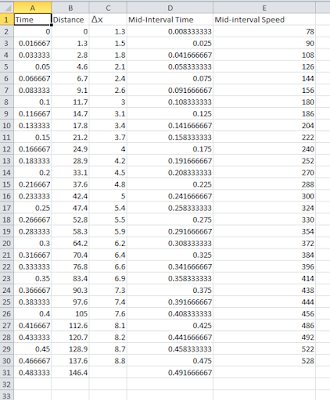
The spark tape is removed and the distance between each mark is measured. These values are our x. The values are input into an Excel sheet. On the same spreadsheet, we make cells for TIME (interval 1/60s), ∆x (difference between consecutive  values of x), mid-interval time (value of time + 1/120), and mid-interval speed (∆x/(1/60)). Then, we generated a mid-interval speed vs mid-interval time graph. The scatter point graph was linearly fit, and the slope should give us the experimental value of g.

Data:

Excel Data Table

Resulting Graph, Linear Fit

The Y-axis is the velocity of the falling spark generator in centimeters per second, while the X-axis is the time in seconds. The slope of this line represents the rate of change in V over time, or ∆v/t, which is the formula for acceleration. The line data shows us that the experimental value of acceleration is 969.69 cm/s^2 or 9.70 m/s^2.

Distance vs Time graph, Polynomial Fit

This graph is different from the first one in that the Y-axis is the value for distance in centimeters, so it becomes a distance vs time graph. The trendline is polynomial fit to the order of two: y=484.09x^2+68.843x-0.0103. This polynomial is in the form of the common kinematics equation 

y=v0t+0.5at^2. We can see that the value with the order of 2 represents 0.5 of a, and the experimental value 484.09 cm/s^2 is roughly half of the known value of g at 981 cm/s^2.

Class Data for g

The class data for this lab

The average class data for the experimental value of g was 961.5 cm/s^2 compared to our own 969.69 cm/s^2. Our standard deviation of the mean was 37.437, calculated by the formula below

Source: http://geographyfieldwork.com/StandardDeviation1.htm

Questions: 

1. Show that, for constant acceleration, the velocity in the middle of a time interval is the same as the average velocity for that time interval.

The velocities at the start of the time interval and the end of the time intervals are the velocities of interest, heretofore called Vi and Vf, respectively. Assuming constant acceleration, the change in velocities is linear and constant between Vi and Vf. That means the value of Vm at the middle of the time interval is equidistant from Vi and Vf  (Vm-Vi = Vf - Vm). Manipulating this equation yields 2Vm = Vf + Vi which yields Vm = (Vf-Vi)/2. Therefore, Vm = Vavg.

2. Describe how you can get the acceleration due to gravity from your velocity/time graph. Compare your result with the accepted value

Because acceleration is the rate of change in velocity over time, the slope of a velocity vs time graph is the value of g, in cm/s^2. Our experimental value of 969.69 cm/s^2 was slightly below the accepted value of 9.81m/s^2 or 981cm/s^2.

3. Describe how you can get the acceleration due to gravity from your position/time graph. Compare your result with the accepted value.

As mentioned above, position and acceleration are detached by an order of two. Using a polynomial trendline on our position vs time graph yielded us y = 484.09x^2+68.843x-0.0103. And because the kinematics formula with a relation between d, t, and a is x = v0t + 1/2(at^2), our value of g/2 is in the coefficient of the term in the second order. 484.09 * 2 = 968.18 cm/s^2, which is slightly lower than the accepted value of 9.81m/s^2.

Conclusion: 

Using the position data gathered from the "free fall" apparatus, we graphed both position vs time and velocity vs time in order to find our experimental value of g. We observed the relationship between position, time, velocity, and acceleration. Our experimental values of g, derived from both position and velocity graphs, were 969.69 cm/s^2 and 968.18 cm/s^2 respectively, slightly lower than the accepted value of 981 cm/s^2. This is most likely due to dissipative forces in the experiment: friction against the wire railing and a slight air resistance. These two forces counter act the force of the weight of the falling object, and the experiment is slightly flawed in that the object does not have an acceleration equal to the value of gravity. Our standard deviation of the mean from class data was 37.437.

Lab 1: Inertial Balance

Jin Im

with Victoria Bravo and Jonathan Goei

27 February, 2017

By using a photogate, series of masses, and an inertial pendulum, we sought the relationship between mass and the period of said pendulum. Once we found this relationship and derive the equation, we measured the period of objects with an unknown mass on the pendulum in order to predict its mass. By graphing the periods of multiple masses on the inertial balance using the given formula T=A(m+M)^n, we seek to find the degree of correlation between period and mass.

The experiment was set up such that the inertial balance, which has a horizontal degree of motion, was attached to the edge of a table. A photogate connected to a laptop, which we used to measure period of oscillations, was placed directly opposite the balance. A thin piece of tape as affixed to the end of the balance, as thinner objects passing through the photogate give us a more accurate period. The apparatus is shown below. 

When an object with mass m is placed onto the stand, as shown, and the system allowed to oscillate, the laptop provided a period T. We replicated this 9 times with different values of m: 0g, 100g, 200g, 300g, 400g, ... etc. 

Using the given formula T=A(m+M)^n, in which M is the mass of the tray oscillating with the masses and A and n are constants, we see that by using different values of m and their corresponding T, we can predict the other values. The formula above was converted to slope-intercept form by taking the natural log of both sides: ln T = n ln(m+M) + ln A. Ln(m+M) becomes our independent variable, ln T becomes our dependent variable, n becomes our slope, and ln A becomes our y-intercept. 

Although the value of M was unknown, we were able to predict it by using a dynamic variable for M in plotting ln T = n ln(m+M) + ln A. By gradually 'sliding' the value of M in the graph, we were able to find the value of M such that the graph had formed a straight line with a correlation coefficient close to 1. Our experimental value for M ranged from 282g to 351g.

Data Table assuming M is 282g

ln T = n ln(m+M) + ln A when M is 282g

282g is the first value for M such that the correlation value on the graph reaches 0.9998,
an acceptable value for the purposes of this lab.

when M is 300g

when M is 351g

These graphs include everything that we need to know to describe the relationship between the mass

and period. Looking at the formula T = A(m+M)^n, we see that n is the slope of the lines of the graphs

above. ln A is the y-intercepts of these lines (A can also be found by T = A(m+M)^n as we now have 

all the variables). The data chart of all relevant values at differing values of M is as shown: 

          For example: T = A(m+M)^n

                                 0.503 = A(400+300)^0.689

                                 0.503 = 91.26A

                                 A = .0053

With these values, we were also able to predict the mass of certain objects by placing them on the apparatus. We used two objects: a small basketball and my TI-83 calculator.

For example, the basketball:

We measured the period of oscillation to be 0.45798 seconds.

0.45798 = .0065(m+ 282g)^0.6695

70.15 = (m+282g)^0.6695

571.9 = m + 282

m = 289.0 grams, assuming M is 282g

0.45798 = .0035(m+351)^0.7499

130.85 = (m+351)^0.7499

664.9 = m+ 351

m = 313.9 grams, when M is 351g 

Our range of mass of the basketball is between 289.0g and 313.9g. The actual value of the ball, as measured on a scale, turned out to be 291g.

The period of oscillation for the calculator was 0.4348s, and the range of mass was from 250g to 269g, while the actual value was 255g. 

Conclusion

The experiment to find the relationship between the mass and period of an object was a roundabout one, with variable values with a degree of uncertainty. Because we had to rely on a range of values for the mass of the tray, the relationship between the mass and period of a inertial pendulum we derived from this experiment is ranged as well. We also performed the experiment with the assumption that the tape attached to the tray of the inertial balance would not sway in the oscillations, which perhaps yielded inaccurate period readings.